---

In this blog post, I wanted to show you how you can monitor the performances of a Bifrost graph, sections of a graph, and even individual nodes. Currently, there isn’t any built-in profiler, or visual timing indicator within Bifrost’s UI, but we still have the ability to monitor performances using Maya’s Profiler. To demonstrate how to do it, I’m going to use the dielectic_ray_visualizer graph from the latest Rebel Pack, which you can download here.

Once you have loaded the graph, let’s hit play and hit the Start Recording button inside Maya’s profiler. Below, you can see a single frame zoom of the Category View. The part we are interested in is called BifrostGraph, and appears in light yellow. Although it is divided in 3 parts, you should only care about the longest one, which represents the total computation time of your graph.

Pretty simple so far, it’s just the same as profiling anything in Maya. But what if we want to profile only a node, a compound or a section of a graph? Bifrost actually have two built in nodes called profiler_start and profiler_end. The way they work is pretty straightforward, but there are some limitations you should know. For exemple, it doesn’t accept any kind data type as input. Complex data types like geoLocation won’t work. It also won’t take any 2D array data types (or with more dimensions).

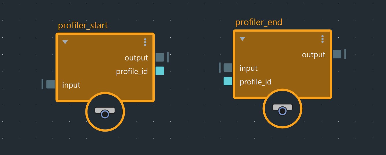
Let’s see how we can use them inside of our graph. In this exemple, I want to know how much time it takes to build the raycast accelerator. All I have to do is just plug the two profiler nodes before and after my accelerator node. You must also plug the profile_id ports together. They are used to know which profiler nodes are associated together.

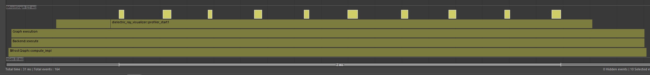
Now, let’s hit play again and check Maya’s profiler window. We can see that another bar appeared on top of the default ones, and we are now able to see how much time the build_raycast_accelerator node takes to compute (in this case, just under 2ms per frame).

We can add as many profilers as we want. Let’s add another one around the iterate_ray_depth compound. In our profiler’s window, we now have another bar that appeared just after the one for our build_raycast_accelerator. As you might notice, the names of the bars in the profiler are a combination of the Bifrost graph’s name + profiler_start. It is not currently possible to set a custom name, which can be a real pain if you plan to monitor multiple nodes at once, so you should definitely keep this in mind when profiling.

Finally, I wanted to show you that you can also profile anything inside loop compounds. I profiled the raycast compound, inside the iterate_ray_depth compound. As it loops 10 times for each frame, the profiler will display an array of 10 smaller bars on top of the pre-existing one.

So that concludes our lesson about using the profiler nodes inside Bifrost. As you can see, there are some downsides, and one can think that it isn’t super user-friendly, but Bifrost still let us have the ability to profile anything in detail, which can be really useful when you want to find where is the bottleneck inside your Bifrost graph.

In our next blog post, we will talk about something I really enjoy, strands ! Stay tuned, and have fun Bifrosting.

Maxime

bifrost compound graph iterate loop maya monitor performance